


Our interactive story, “Hell and High Water,” includes a map with seven animated simulations depicting a large hurricane hitting the Houston-Galveston region. Four of the scenarios depict a hurricane hitting with existing storm protection infrastructure in place; three envision storm protection projects proposed by a number of universities in Texas.
Five of the simulations were developed by teams at the University of Texas at Austin, and the Severe Storm Prediction, Education and Evacuation from Disasters (SSPEED) Center at Rice University.
- A re-creation of Hurricane Ike, a real storm that hit Texas in September 2008.
- Storm P7, a simulation that envisions Hurricane Ike making landfall near San Luis Pass, about 30 miles southwest of where it actually landed. According to Dr. Phil Bedient at Rice, the chances of the Storm P7 scenario occurring in any given year is about one in 100.
- Storm P7+15 (a.k.a. “Mighty Ike”), which follows the same path as the P7 storm, but with 15 percent higher wind speeds. Bedient told ProPublica and The Texas Tribune that the chances of the Storm P7+15 scenario occurring in any given year is one in 350.
- Mid-Bay Scenario, which simulates the P7+15 storm but includes a gate across the middle of Galveston Bay that would prevent storm surge from reaching Clear Lake and the Houston Ship Channel. The Mid-Bay scenario was proposed by the SSPEED Center at Rice University.
- Coastal Spine, which simulates the P7+15 storm but includes a proposed 17-foot wall along Galveston Island and the Bolivar Peninsula, and a gate across Bolivar Roads, which would prevent storm surge from entering Galveston Bay. The Coastal Spine is a version of a proposal by Dr. William Merrell at Texas A&M-Galveston.
Two simulations are based on synthetic storms developed by the Federal Emergency Management Agency as part of the RiskMAP flood mapping study and modeled by researchers at Jackson State University. Synthetic storms, as opposed to the P7 storms that were based on Hurricane Ike, never appeared in nature, but are derived from averaging hundreds of actual storms that have hit the Texas coast.
- Storm 36 is a synthetic storm that, like some other scenarios, makes landfall near San Luis Pass. According to JSU researchers, the chances that Storm 36 will occur in any given year is 1 in 500.
- Coastal Spine (extended) simulates Storm 36 as if it were protected by a 17-foot-tall structure similar to the Coastal Spine, except it extends as far as Sabine Pass to the Northeast and as far southwest as Freeport. The “extended” Coastal Spine is the current version of the Coastal Spine/Ike Dike proposal by Dr. William Merrell at Texas A&M Galveston.
Researchers provided all of the storm data to ProPublica and the Texas Tribune in formats used by the ADCIRC system. Run on powerful supercomputers at UT-Austin and the U.S. Army Engineer Research and Development Center’s Coastal and Hydraulics Laboratory (ERDC), ADCIRC takes a variety of storm inputs and is able to derive storm surge, wind strength and wind vectors with high precision, even over local areas. ProPublica and the Texas Tribune worked primarily with three ADCIRC file formats: a fort.14 grid file, a fort.63 water elevation time series file, and a fort.74 wind vector time series file.
The fort.14 grid is a highly accurate 3-D height map of the Texas coast. The grid provided to ProPublica and the Texas Tribune by Dr. Jennifer Proft at UT-Austin was created in 2008 and contains about 3.6 million points. The fort.63 and fort.74 files provided by UT are hourly snapshots during simulated storms starting on Sept. 11, 2008 at 1 p.m. UTC and continuing for 72 hours.
The grid files provided to us by Jackson State University that depict Storm 36 and Storm 36 protected by the “coastal spine” structure are each roughly 6.6 million points (though, within our areas of interest, the JSU and UT grids have about the same number of points). The Storm 36 time series files start on the fictitious date of Aug. 2, 2041 at 10:30 a.m. and continue for 96 hours in half-hour time steps. The Storm 36 (with Coastal Spine) time series files begin on the fictitious date of Aug. 1, 2041 at 1:30 a.m. and continue for 94 hours in half-hour time steps.
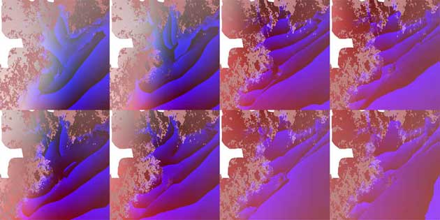
The ADCIRC grids are what are called “unstructured grids,” meaning the resolution varies at different locations in the mesh. The length of the lines connecting grid nodes varied from about 50 meters to about 1,000 meters within our areas of interest. Because of this variability, the resolution of any given triangle ranges from about 1,250 square meters to about 45,000 square meters.

Variation in grid resolution in roughly our areas of interest (Jackson State University)
Additionally, the water surface elevations in the fort.63 files have a margin of error of about 1-2 feet, according to Bruce Ebersole at Jackson State University.
To display all of these storms on the same timeline, we synchronized the landfall of all the storms around Hurricane Ike’s landfall on Sept. 13, 2008 at 7 a.m. UTC. To account for varying lengths of the time series files between all of the storms we wished to show our timeline, we synchronized our storm simulations to begin at 16 hours before landfall, and continue until 24 hours after landfall. Because the storms provided to us by Jackson State University are saved in half-hour time steps and the UT storms are saved in hour time steps, we removed every other snapshot from the Jackson State storms before processing them for our interactive graphic.
Our application focused on an initial 160km-by-120km area of interest surrounding the Houston/Galveston area and smaller areas covering the Houston Ship Channel (32km by 15km), Clear Lake (23km by 20km) and Galveston (9km by 6km).
Processing ADCIRC into PNGs
In order to process the ADCIRC files for display on the web, we had to compress the massive size of the initial datasets provided to us. To do that, we developed a processing pipeline that broke the grids and time series down first into our areas of interest, and then encoded averaged data into the red, green, blue and alpha channel pixels of PNG images for fast delivery to the browser.
First, we used an ADCIRC Fortran utility program called resultscope to “crop” the fort.14, fort.63 and fort.74 files to all of our areas of interest. This cut our “background” area, for example, down to a grid of about 650,000 points. We took these resulting files and encoded them into a series of data-encoded images. For each area (the “background,” the Houston Ship Channel, Clear Lake and Galveston), we created a 512×512 pixel PNG image and “packed” the height data into the RGBA values of the image using OpenGL and Ruby. In these “image databases,” we encoded green value to the height of the grid at a pixel location, the blue to the height after the decimal, and the red byte as a flag indicating whether the point was above or below sea level (NAVD88).
In order to format this data efficiently for transport over the Internet and manipulation in a web browser, we also “packed” each hour of the time series into PNG images, with the red and alpha values storing the wind x and y vectors respectively, the green value containing the water height at the location and the blue value containing the height of the water after the decimal. To further optimize the images for delivery over the web, we composited the time series images into sets of 1024×1024 images each containing four 512×512 images. Each storm, therefore would be a single 512×512 grid image, and ten 1024×1024 time series images, comprising 40 hours of the storm. In the application, we have seven sets of those images (for each storm), for every area of interest. The entire app is comprised of 28 sets or 308 images total. (If we had not collected the time series into quadrant images, there would have been 1,148 images altogether.)
Because every storm was compressed into the same 512×512 resolution, the accuracy of each area of interest varies. For the background, the accuracy is averaged over 72,072 square meters, for the Houston Ship Channel View, 1,932 square meters, for Clear Lake, 1,803 square meters, and for Galveston, 231 square meters.
Since the grid resolution varies at different points around the mesh, even though every pixel of our “image databases” is averaged over the same area, the underlying data may be lower resolution:

Resolutions of elevation in the real world, the ADCIRC grid, and our PNG “image databases” (Illustration: Sarah Way for ProPublica)
Our interactive graphic uses WebGL to decode these images in the browser and display the animations to the reader. In the graphic, the base image shown to the reader is a pan-sharpened true-color Landsat image of the Texas Coast. Using WebGL, we then mixed blue (rgba(18, 71, 94, 1)) into the satellite image in areas where the depth of the grid was below sea level or the surge exceeded the underlying elevation over the course of the time series.
Because it wouldn’t be a hurricane without wind, we created a particle system to show the wind direction and speed. We worried that showing large amounts of particles on the vizualisation would slow the animation to a crawl, but we found a WebGL extension called instanced arrays that makes copies of just one instance of our particle and efficiently draws it thousands of times. The particles are randomly placed small rectangle meshes, and we rotate each rectangle based on the wind data in each storm’s underlying “image database.” For every frame we also update the rectangle’s position based on the wind velocity at that point, which we store in a WebGL texture. Each wind particle only lives for about a second before it fades out and resets to it’s original position. The wind speed in the visualization is 20 times as fast as in the underlying computer model because even hurricane sized wind speeds when viewed from what is essentially space would be imperceptible.
We presented other metadata about the storms, such as the storm tracks, and proposed and existing storm protection measures on the map as vector data. Texas A&M Galveston provided the current “extended” Coastal Spine scenario to ProPublica and the Texas Tribune as a low resolution raster image, which we converted into a vector file. Although it is therefore imperfect it is our best estimate of what that conception of the Coastal Spine would look like.
Rice University, via UT-Austin, provided the other proposed and existing barriers to us as a shapefile. UT-Austin provided the storm tracks for Ike, P7, and P7+15 as a shapefile and we converted them into GeoJSON. Jackson State University provided the storm track for storm 36 as a ” TROP file.” We synchronized it to the “Ike” timeline and converted it to a GeoJSON to present on the map.
The storage tanks presented in the Houston Ship Channel view come from a database created by Dr. Hanadi Rifai, and others, at University of Houston. To create that dataset, University of Houston researchers scrutinized 2008 aerial images to classify the tanks. The storage tank data is therefore current as of 2008.
Several other features in the interactive graphic use the same PNG “image database” we created to present the storms, including the address-lookup function and the surge numbers at Galveston Strand, Johnson Space Center and ExxonMobil Chemical. However, this process is done server-side, because we discovered that querying pixel data in the browser using the getImageData method in canvas returns incorrect results for images with alpha transparency.
The timeline graph at the top of the page is also generated by querying this same PNG “image databases” for each storm and area of interest at a given point. The point depicted in the timeline graph changes based on the area of interest: The overview as well as the Clear Lake area of interest depicts a point near the Kemah Boardwalk; the Galveston AOI is a point on the Galveston Strand; and the Houston Ship Channel view is a point on the ExxonMobil Chemical facility near 5000 Bayway Drive, Baytown, Texas.
We used Google’s address geocoder. The accuracy of these numbers is the same as the resolution of the areas of interest noted above.
We would like to extend our thanks to the teams at Rice, UT-Austin, Texas A&M Galveston and Jackson State University for helping us understand and present this data, especially Jennifer Proft at UT and Bruce Ebersole at Jackson State University, who have spent many hours patiently guiding us through the intricacies of storm data.


